Practical Statistics for Data Scientists

Ordinal: Categorical data that has an explicit ordering

Records: A row in the table (dataset)

Rectangular data: Data in a table form

Non-Rectangular data structure: 1) Spatial data (it stores data indexed in some way by their spatial location), 2) Graph data structure

Trimmed mean: It's a compromise between median and mean. The front and back ends are dropped (trimmed) by $n%$ (usually, $10%$) and the mean is calculated. It's robust to outliers and widely used.

Deviation: Error, residual

Variance and standard deviation are sensitive to outliers. The more robust metric for the variability is median absolute deviation (MAD) and trimmed standard deviation which is analogous to the trimmed mean.

$ MAD = Median( |x_1 - \bar{x}|, |x_2 - \bar{x}|, \cdots, |x_n - \bar{x}| ) $

Correlation coefficient is sensitive to outliers. So, calculating the coefficient of the trimmed data is more robust to outliers.

Hexagonal Binning and Contour

Scatter plots are fine when there is a small number of data. For datasets with a lot of records, a scatter plot will be too dense. Thus, we use the Hexagonal Binning and Contour.

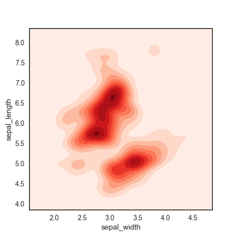
Left: Hexagonal plot, Right: Contour plot where each contour band represents a specific density of points ($\approx$ count)

 

Contingency Table

Useful to summarize two categorical variables. For instance, records of a Poker player with three different croupiers can be presented as:

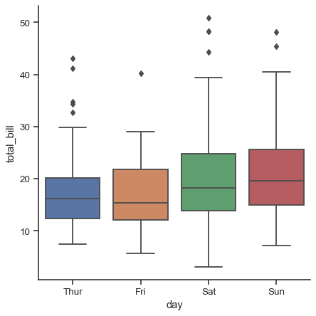
The cells are filled with frequencies (= counts). It would be efficient to visualize it with a heatmap

Box Plot

It is a simple way to visually compare the distributions of numeric variables grouped according to a categorical variable.

Conditioning

The types of charts used to compare two variables - scatter-plot, hexagonal binning, and box plot, are readily extended to more variables through the notion of conditioning. For example,

Left: Before the conditioning, Right: After the conditioning w.r.t smoker

Statistical Moments

• First moment: Location (e.g. mean)
• Second moment: Variability (e.g. standard deviation)
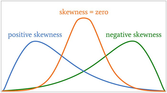
• Third moment: Skewness
• Fourth moment: Kurtosis, which defines how heavily the tails of a distribution differ from the tails of a normal distribution. In other words, kurtosis identifies whether the tails of a given distribution contain extreme values.

Note that the third and fourth moments are not commonly written numerically. Rather, they are presented by chards (graphs).

Selection Bias

It refers to the practice of selectively choosing data - consciously or unconsciously - in a way that that leads to a conclusion that is misleading. Typical forms of selection bias are:

• Vast search effect: Results from repeated data modeling or modeling data with large numbers of predictor variables.
• Non-rando sampling: 실험참가자를 그냥 공고내서 모집하여 모은 실험참가자들은 possibly biased. because 지원해서 참가를 한 ㅅ람은 자발적으로 참가하지않은 사람들과 성향이 다른 사람일수 있기 때문.
• Selection of time interval that accentuate a particular statistical effect
• Data snooping: Extensive hunting through data in search of something interesting.

Regression to the Mean

mean값에서 벗어난 값들은 머지않아 mean 값으로 다시 돌아온다. For example, 한 야구선수가 1년차에 운이 좋아 실적이 엄청났다면, 2년차에는 실적이 떨어진다 (= 즉, 평균으로 돌아옴), 또는 Stock prices.

Data Distribution v.s Sampling Distribution

• Data Distribution: Distribution of individual data points
• Sampling Distribution: Distribution of sample statistic

Bootstrap / Bootstrapping

It is one easy and effective way to estimate the sampling distribution of a statistic by drawing additional samples with replacement from the sample itself. The steps of the bootstrapping are as follows:

1. Draw a sample value, record, with replacement.
2. Repeat $n$ times.
3. Record the mean of the $n$ resampled values.
4. Repeat the steps 1-3 $R$ times. (as a rule of thumb, you can start trying $R$ of 10,000)
5. Use the $R$ results to : a) Calculate the standard error (SE), b) Produce the sampling distribution

The bootstrap can be used with multivariate data, where the rows are sampled as units. Some statistical model might be run on the bootstrapped data.

With a decision tree, running multiple trees on bootstrap samples and then averaging their predictions (or taking a majority vote for classification) generally performs better than using a single-tree. This process is called bagging (bootstrap + aggregating).

It is popular for the use with metrics or models where mathematical approximations are not readily available. 

It does not rely on the Central Limit Theorem or other distributional assumptions.

The real question we are interested using the central limit theorm and the bootstrapping is "Given a sample result, what is the probability that the true value lies within a certain interval?"

Normal Distribution

It is a common misconception that the normal distribution is called that because most data follows a normal distribution. Actually, most data do not follow this. Its name derives from the fact that many statistics are normally distributed in their sampling distribution.

Long-Tailed Distribution

Tail: The long narrow portion of a frequency distribution, where relatively extreme values occur at low frequency.

Black Swan Theory: It predicts anomalous events.

t-Distribution

Distributions of sample means are typically shaped like the t-distribution. If the sample size $n$ is large, the t-distribution resembles the normal distribution.

Exponential Distribution

Distribution of the time between events (= a statistical distribution that models the time between events). For example, 1) Time between visits to a website, 2) Time between cars arriving at a toll plaza.

Its formula is $ Pr = \lambda e^{- \lambda x}$ and its general shape of the distribution is:

$\lambda$ in the exponential distribution has the same meaning as in the Poisson distribution

Note that the exponential distribution has one parameter - $\lambda$ (= #occurences / specified period)

How to determine $\lambda$ for the exponential distribution? For example, 

• a) Someone watches this video at every 0.5s on average: $\lambda = 2$ [#occurences / 1s]
• b) Someone watches this video at every 1s on average: $\lambda = 1$
• c) Someone watches this video at every 2s on average: $\lambda = 0.5

Weibull Distribution

If the period over which the event rate changes is much longer than the typical interval between events, there is no problem; you just subdivide the analysis into the segments where rates are relatively constant. If, however, the event rate changes over the time of the interval, the exponential (or Poisson) distributions are no longer useful. This is likely to be the case in mechanical failure - the risk of failure increases over time.

The Weibull distribution is an extension of the exponential distribution, in which the event rate can be specified by a shape parameter $\beta$ (or $\lambda$) and the characteristic life can be specified by a scale parameter $\eta$ (or $k$). The shape of the Weibull distribution w.r.t the scale parameter is:

Note that when the scale parameter is 3.26, the Weibull distribution is very close to the normal distribution

Statistical Experiments and Significance Testing

1. The classical statistical inference pipeline is:
2. Formulate hypothesis 
3. Design experiment
4. Collect data
5. Inference (it reflects the intention to apply the experiment results, which involve a small set of data, to a large process or population.)

A/B Testing

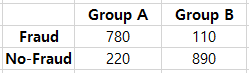
A/B testing is an experiment with two groups to establish which of two treatments, products, procedures, etc. is superior. The most common test statistic to compare 'group A' to 'group B' is a binary variable. For instance, (click or no-click), (buy or no-buy), and (fraud or no-fraud). Those results would be summed up in a $2 \times 2$ table:

Why Just A/B? Why not C, D, $\cdots$ ?

We are often interested in "out of multiple possible groups, which is the best?". For this, a relatively new type of experimental design is used, called Multi-Arm Bandit.

Hypothesis Test

The hypothesis test is a further analysis of the A/B test or any randomized experiment to assess whether random chance is a reasonable explanation for the observed difference between groups A andB.

Resampling

Resampling in statistics means to repeatedly sample values from observed data with a general goal of assessing random variability in a statistic. There are two main types of resampling procedure: 1) Bootstrap, 2) Permutation Test. The permutation tests are used to test hypotheses. Its procedure is as follows:

1. Specify $H_0$ and $H_1$. (For example, weight gain is irrelevant to a diet, in which 'Group A': 채식, 'Group B': 육식)
2. Choose a test statistic. e.g. $\mu_A- \mu_B$ or |MED_A - MED_B| where $MED$ refers to the median.
3. Compute a distribution of the test statistic using the permutations of the observed data.
4. Compute $p$-value (= #permutation test statistic that are greater than the observed test statistic / #total permutations)
5. If $p$-value $<$ the significance level $\alpha$, we can reject $H_0$.

Note that the distribution of the permutation test statistics usually follows the t-distribution.

Proxy variable

One that stands in for the true variable of interest, which may be unavailable, too costly, or too time-consuming to measure. For example, in climate research, the oxygen content of ancient ice cores is used as a proxy for temperature.

Exhaustive Permutation Test and Boostrap Permutation Test

• Exhaustive Permutation Test: 보통의 permutation test에서는 $R$개의 permutations을 생성하여 테스트를 진행하는데, 이는 모든 permutation의 경우를 다 고려하기엔 computationally expensitve하기 때문이다. 하지만, 작은 데이터셋에 대해선 모든 permutation의 경우를 전부 고려할 수 있다. 이를 exhaustive permutation test라고 부른다.
• Bootstrap Permutation Test: 일반적인 permutation test에서는 permutation 생성시 'without replacement' 를 사용한다. 'with replacement' 를 사용한 경우를 bootstrap permutation test 라고 한다.

$p$-Value

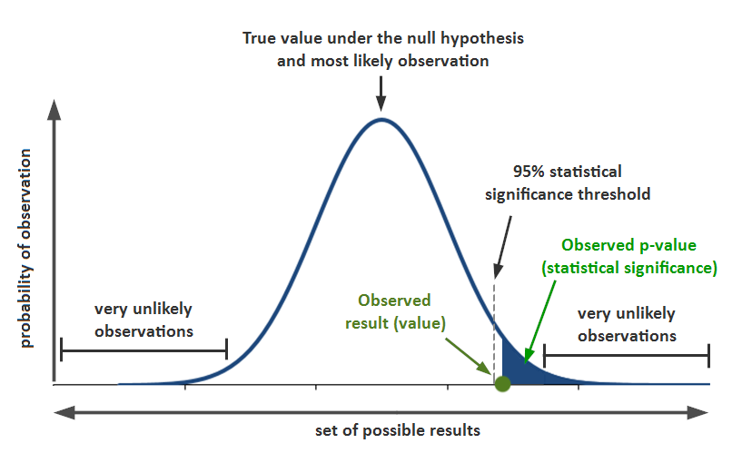
The $p$-value is the probability calculated by the shaded area

t-Test

옛날 1920, 1930년대에는 컴퓨터 성능이 좋지않아, distribution of permutation test statistics을 구하는게 어려웠다, 그래서 찾아낸게 t-distribution으로  distribution of permutation test statistics를 잘 근사할 수 있다는 사실이다. 그래서 옛날에는 permutation test 대신 t-test (t-distribution을 이용함) 를 하였다. 근래에, bootstrapping이나 permutation test를, central limit theorem 이나 t-test보다 더 선호하는 이유는 다음과 같다: 1) 여러 가정이 필요없음. 예를 들면, 데이터가 특정 distribution을 따른다. Center limit theorm은 $\bar{X}$ \sim N(\mu, \frac{\sigma^2}{n})$을 가정하고, t-test는 permutation test statistic이 t-distribution을 따른다고 가정한다.

Multiple Testing

For example, if you have 20 predictor variables and one output variable, all randomly generated, the odds are pretty good that at least one predictor will (falsely) turn out to be statistically significant. If you do a series of 20 significant tests at $\alpha = 0.05$. This is called the Type 1 error.

The probability that one will correctly test non-significant is $0.95$, so the probability that all 20 will correctly test non-significant is $0.95^{20} = 0.36$. Then, the probability that at least one predictor will (falsely) test significant is $1-0.36 = 0.64$.

The main issue in the multiple testing is that the more variables you add, or the more models you run, the greater the probability that something will emerge as significant just by chance.

To compensate for that, there is an adjustment procedure: Dividing up $\alpha$ by a number of tests.

Degrees of Freedom

It refers to a number of values free to vary. For example, if you know the mean of a sample of 10 values, and you also know 9 of the values, you also know the 10th value. Only 9 are free to vary. 

When sample statistics are standardized for use in traditional statistical formulas, degrees of freedom is part of the standardization calculation to ensure that your standardized data matches the appropriate reference distribution such as t-distribution, F-distribution, etc.

ANOVA

There are two approaches:

• Formula Approach (traditional). 
• Resampling Approach (modern, more exact). 

Refer to my blog posting about ANOVA for the above two approaches.

F-Statistics

To use the formula approach for ANOVA, we need the F-statistic (F-ratio). It is based on a ratio of the variance across group means to the variance due to residual error.

Chi-Square Test

Two main purposes of $\chi^2(v)$ are

1. To test if an observed distribution follows an expected distribution.
2. To test a null hypothesis of independence among variables.

For example, here is an example data:

and we assume that we already know the expected distribution. We can do the chi-square test in the following manner:

1. Constitute a box with 34 ones (clicks) and 2,966 zeros (no-click).
2. Shuffle, take three separate samples of 1,000, and count the clicks in each.
3. Find the squared differences between the shuffled counts and the expected counts, and sum them; $\sum_{k}{(observed \: - \: expected)^2}$
4. Repeat steps 2-3, say, 10,000 times.
5. Calculate $p$-value (= (#times that the resampled sum squared deviation > the observed sum squared deviation) / #total repeatition ) 
6. If $p$-value $<$ $\alpha$, you can reject the null hypothesis, otherwise, you cannot.

Fisher's Exact Test

It is a kind of the permutation test where all the possible permutations are considered. One data science application of the chi-square test, especially Fisher's exact test, is in determining appropriate sample size.

Multi-Arm Bandit Algorithm

The traditional A/B test has a presumption that once we get an answer, the experimenting is over and we proceed to act on the results. It comes with several difficulties: 1) Our answer may be inconclusive; effect not proven, 2) We might want to begin taking advantages of results that come in prior to the conclusion of the experiment, 3) We might want the right to try something different based on additional data.

Bandit algorithms allow you to test multiple treatments (e.g. headline A in a web test is one of the treatments) at once and reach the conclusion faster than traditional statistical design.

Example: There are three slot machines, A, B, and C. The winning is the same but we do not know the probabilities of winning for A, B, and C. How can we figure them out while balancing between exploitation and exploration? $\rightarrow$ We can use Multi-Arm Bandit Algorithm. Its basic concept is as follows:

1. Initially, we pull A, B, and C randomly (equally-random).
2. If A starts winning more, we pull A more often (exploitation), but we do not abandon B and C (exploration).
3. But, later, if C starts winning more, we can shift pulls from A to C. 

What pull rate should we change to, and when should we change? There are mainly two approaches for that:

• Epsilon-greedy approach: Let a random value $r$; $ \left\{ \begin{array}{ll} explotation \quad if \quad r > \epsilon \\ exploration \quad otherwise \end{array} \right. $
• Bayesian approach

Power Calculation / Power Analysis

Refer to my blog posting about power and sample size.

Multiple Linear Regression

$$ Y = b_0 + b_1 X_1 + b_2 X_2 $$

For instance, 아파트가격 = $b_0$ + $b_1$아파트크기 + $b_2$화장실 갯수, which is interpreted as 아파트크기가 1$m^2$ 증가할때마다, 아파트 가격이 $b_1$만큼 증가함. 화장실 갯수가 1개 증가할때마다, 아파트 가격이 $b_2$만큼 증가함.

Assessing the Regression Model

The two most common matrices are 1)RMSE (Root Mean Squared Error), 2) R-squared score $R^2$.

Model Selection and Stepwise Regression

Stepwise Regression: 1) Forward selection, 2) Backward selection.

• Forward selection: You start with no predictors and add them one-by-one, stopping when the contribution to $R^2$ is no longer statistically significant.
• Backward selection: Opposite to the forward selection.

Note that these two approaches are possibly subject to overfitting.

Confidence Interval and Prediction Interval

The confidence interval is an interval of good estimates of the unknown true population parameter. About a 95% confidence interval for the mean, we can state that if we would repeat our sampling process infinitely, 95% of the constructed confidence intervals would contain the true population mean. (source: here)

The prediction interval is an estimate of an interval in which a future observation will fall, with a certain confidence level, given the observations that were already observed. About a 95% prediction interval, we can state that if we would repeat our sampling process infinitely, 95% of the constructed prediction intervals would contain the new observation. (source: here)

(Left) Data is in one dimension. (Right) The grey shaded area denotes the confidence interval and the red dashed line denotes the prediction interval

The confidence interval can be found using the bootstrap:

1. Get a bootstrap sample from the existing data.
2. Fit a regression model to the bootstrap sample, and record the estimated coefficients.
3. Repeat steps 1-2, say, 1,000 times.
4. You now have 1,000 bootstrap values for each coefficient; Find the appropriate percentiles for each one.

The computation of the confidence interval is simulated here in GoogleColab using a linear regression model. The results are as follows:

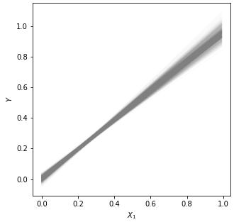
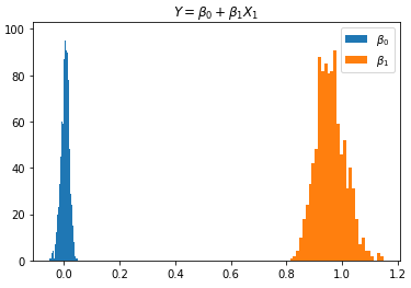
Left: Example data, Middle: 1,000 overlapped models, Right: frequencies of the predictor variables

Instead of the bootstrapping approach, there exists a formula approach to obtain the confidence interval.

Factor Variable with Many Levels

Let's say there is 'zip-code' feature that has 82 levels (= 82 types of zip code). Applying the one-hot encoding will result in 82 columns. Here is what we can do:

1. Remove the zip-code levels where the count is low/small.
2. Group the zip-code into several subgroups (w.r.t something like a proxy variable - housing price).

Ordered Factor Variable

For instance, 만족도 = {매우불만족, 불만족, 보통, 만족, 매우만족} can be converted into numeric values, 만족도 = {0, 1, 2, 3, 4}.

Correlated Preditors

Having correlated predictors can make it difficult to interpret the sign and value of regression coefficients.

Multicollinearity

An extreme case of correlated variables produces multicollinearity - a condition in which there is redundancy among the predictor variables. Perfect multicollinearity occurs when one predictor variable can be expressed as a linear combination of others. The multicollinearity occurs when: !) a variable is included multiple times by error, 2) $P$ dummies, instead of $P-1$ dummies, are created from a factor variable, 3) Two variables are nearly perfectly correlated with one another.

Cofounding Variables

It refers to a very important variable. If it is missing in a regression model, the performance drops significantly. For instance, 아파트크기 can be a cofounding variable to predict 아파트가격.

Interactions and Main Effects

$$ Y = b_0 + b_1 X_1 + b_2 X_2 + b_3 X_1 X_2 $$

The term $b_3 X_1 X_2$ consideres the interaction between $X_1$ and $X_2$.

Outliers

There are rules of thumb for how distance from the bulk of data an observation needs to be in order to be called an outlier; For example, with the box plot, 양쪽 1.5IQR 범위를 벗어나면 outlier로 칭함.

In regression, the standardized residual is the metric that is typically used to determine whether a record is classified as an outlier. The standardized residual is residuals divided by an estimate of its standard deviation.

Influential Values

The influential value is a value whose presence or absence makes a big difference in the regression equation. The leverage is a degree of influence that a single record has on a regression equation.

A metric to measure the influence is Cook's distance. The Cook's distance $D_i$ of observation $i$ (for $i = 1, \cdots, n$) is defined as the sum of all the changes in the regression model when observation $i$ is removed from it.

$$ D_i = \frac{ \sum_{j=1}^n ( \hat{y}_i - \hat{y}_{j(i)} )^2 }{ ps^2 } $$

where $\hat{y}_{j(i)}$ is the fitted response value obtained when excluding $i$, $s^2 = (\boldsymbol{e}^T \boldsymbol{e})/(n-p)$ is the mean squared error of the regression model, and $p$ is a number of learnable parameters.

For the purpose of anomaly detection, it can be useful.

Heteroskedasticity, Non-normality, and Correlated Error

Heteroskedasticity is a lack of constant residual variance across the range of the predicted values.

The residual increases over X

Partial Residual

Partial residual = Residual + $\hat{b}_i X_i$

Splines

A series of piecewise continuous polynomials. The polynomials pieces are smoothly connected at a series of fixed points in a predictor variable, referred to as knots. The spline has two parameters: 1) Degree of the polynomial, 2) Location of knots.

Generalized Additive Models (GAM)

A technique to automatically fit a spline regression.

Naive Bayes

Refer to my blog about Naive Bayes.

Linear Discriminant Analysis (LDA)

Refer to my blog posting for LDA.

Logistic Response Function

Logistic response function: We map a probability (0-1 range) to a more expansive scale suitable for linear modeling. Let's say, we have a linear regression model: $\hat{y} = b_0 + b_1 x_1 + \cdots + b_p x_p$. Then, the logistic response function is:

$$ Pr = \frac{1}{1 + e^{ - \hat{y} }} $$

Maximum Likelihood Estimation (MLE)

The goal of MLE is to find a set of parameters that maximizes the value of $P_{\theta} (X_1, X_2, \cdots, X_n)$ where $P_{\theta}$ refers to a probability with respect to a parameter $\theta$. IN the fitting process, the model is evaluated using a metric called deviance:

$$ deviance = -2 \log{ ( P_{\hat{\theta}} (X_1, X_2, \cdots, X_n) ) } $$

Evaluating Classification Models

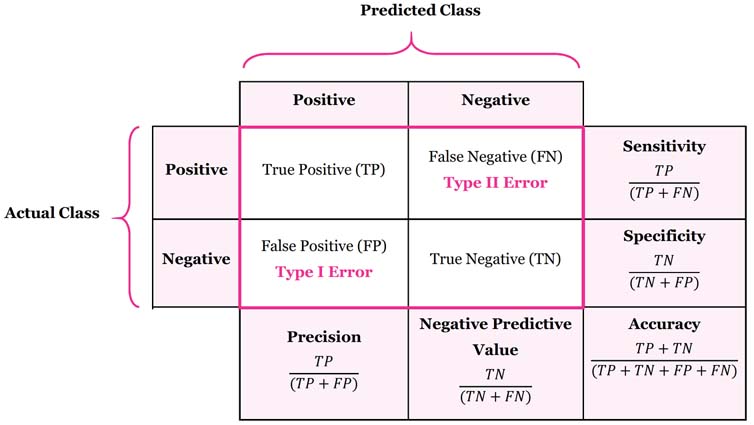
Confusion Matrix. Note that sensitivity = recall

ROC curve. Note that False positive rate = Specificity, True positive rate = Sensitivity

Strategies for Imblalanced Data

• Understampling
• Oversampling: You can ovversample rarer calss by drawing additional rows with replaement.
• Data Generation: e.g. SMOTE

Distance Metrics

• Euclidean distance
• Manhattan distance
• Mahalanobis distance

Refer to my blog posting about distance metrics.

KNN as a Feature Engine

The KNN can be used to add local knowledge in a staged process with other classification techniques. The KNN is run on data, and for each record, a classification (or quasi-probability of a class) is derived. That result is added as a new feature to the record.

The Recursive Partitioning Algorithm

The algorithm to construct a decision tree, called recursive partitioning, is straightforward. The data is repeatedly partitioned using predictor values that do the best job of separating the data into relatively homogeneous partitions, where the homogeneity is measured by impurity metrics. 

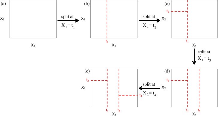
Illustration of the recursive partitioning algorithm

Partitioning algorithm:

1. For each predictor variable $X_j$,
   1. For each split value $s_j$ of $X_j$:
      1. Split the records in a dataset $A$ with $X_j < s_j$ as one partition, and the remaining records where $X_j \ge s_j$ as another partition.
      2. Measure the homogeneity of classes within each partition of $A$.
   2. Select the split value $s_j$ that produces maximum within-partition homogeneity of class.
2. Select the variable $X_j$ and the split value $s_j$ that maximizes within-partition homogeneity of class.

Recursive part:

1. Initialize $A$ with the entire dataset.
2. Apply the partitioning algorithm to split $A$ into two subpartitions, $A_1$ and $A_2$.
3. repeat step 2 on subpartitions $A_1$ and $A_2$.
4. The algorithm terminates when no further partition can be made that sufficiently improves the homogeneity of the partitions.

Measuring Homogeneity or Impurity

1) Entropy, 2) Gini impurity

Refer to my blog posting about the impurity metrics.

Bagging and Random Forest

Refer to my blog posting about ensemble, bagging, and random forest.

Variable Importance

1. By the mean decrease in the Gini impurity score.
2. By the decrease in accuracy of the model if the values of a variable are randomly permuted.

The first approach is a byproduct of the algorithm. It is easy to get, but less accurate. The second approach requires some computation but more accurate.

Boosting Algorithm

Refer to my blog posting about Boosting.

PCA

PCA를 돌리면 ($\approx$ SVD), principal components (= eigenvectors)를 가지는데, 이것을 해석하는게 데이터에 대한 intuition을 줄 수 있다. 예를들면, principal component (PC) #1 = $\begin{bmatrix} 0.63 \\ 0.77 \end{bmatrix}, 이라면 1st row는 1st feature의 PC1에 대한 영향력을 나타내고, 2nd row는 2nd feature의 PC1에 대한 영향력을 나타낸다.

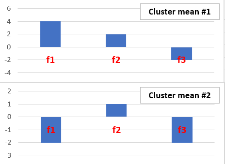
Interpreting the Clusters

Cluster mean들의 vector값을 Bar graph로 나타내어 해석가능하다.

Hierarhical Clustering

Refer to my blog posting about hierarchical clustering and agglomerative algorithm.

Model-Based Clustering

The techniques are grounded in statistical theory and provide more rigorous ways to determine the nature and number of clusters. The most widely used model-based clustering methods rest on the multivariate normal distribution (refer to my blog posting about the multivariate normal distribution). 

The key idea behind model-based clustering is that each record is assumed to be distributed as one of $K$ multivariate-normal distributions, where $K$ is the number of clusters. Each distribution has a different mean and covariance matrix. For example, if you have two variables, $X$ and $Y$, then each row $(X_i, Y_i)$ is modeled as having been sampled from one of $K$ distributions $N_1(\mu_1, \Sigma_1)$, N_2(\mu_2, \Sigma_2), \cdots, N(\mu_K, \Sigma_K)$. The number of clusters is chosen such that the Bayesian Information Criteria (BIC) is the largest.

An example of the model-based clustering is shown below, where the stock return data is used:

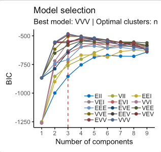
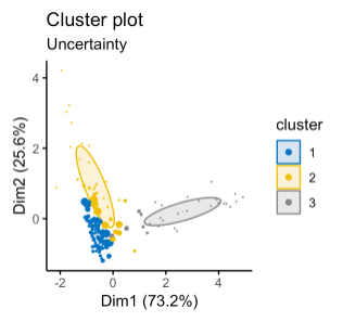
Left: BIC scores for different numbers of clusters and different models. Middle: Classification cluster plot. Right: Uncertainty cluster plot, where the larger symbols denote greater uncertainty.

where the model names in the left-hand figure are interpreted as follows: 

Interpretation of the model names 

Model-based clustering techniques do have some limitations. The methods require an underlying assumption of a model for the data, and the cluster results are very dependent on that assumption The computations requirements are higher than even hierarchical clustering, making it difficult to scale to large data.

Gower's Distance

Refer to my blog posting about Gower's distance.

Problem with Clustering Mixed Data

In practice, using k-means and PCA with binary data can be difficult because if the standard z-scores are used for scaling, the binary variable will dominate the definition of clusters.

To avoid this behavior:

1. Scale the binary variables to have a smaller variance than others.
2. Apply clustering to different subsets of data taking on specific categorical values.