Gower's Distance

It measures the dissimilarity between records within a mixed dataset. The mixed dataset refers to a dataset where both a numeric feature (variable) and a categorical feature (variable) exist together.

The basic idea behind Gower's distance is to apply a different distance metric to each variable depending on the type of data:

• For numeric variables and ordered factors (ordered categorical variable), distance is calculated as the absolute value of the difference between two records (Manhattan distance).
• For categorical variables, the distance is 1 if the categories between two records are different and the distance is 0 if the categories are the same (Dice distance).

The mathematical formula for the Gower's distance is:

$$ S_{ij} = \frac{\sum_k{w_{ijk} S_{ijk}}}{ \sum_k w_{ijk} } $$

where $S_{ij}$ is the dissimilarity matrix w.r.t records, $S_{ijk}$ is the dissimilarity matrix of a $k$-th variable w.r.t records, $w_{ijk}$ is weight for each dissimilarity matrix $S_{ijk}$.

Algorithm by Example

Let's say we have the following example dataset:

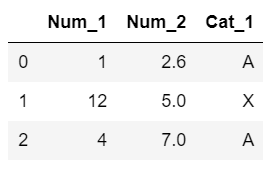
Dataset

Since there are three records, our dissimilarity matrix $S_{ij}$ and $S_{ijk}$ will be $3 \times 3$ matrices. Here are the simple steps for the algorithm:

1. Compute three $S_{ijk}$ where $k=1, 2, 3$ since there are three variables.
2. Add $S_{ij1}, S_{ij2}, S_{ij3}$ together, either using a simple mean or weighted mean.

Note that the Manhattan distance is used for the numeric variables and the dice distance is used for the categorical variable.

First, we compute $S_{ij1}$ by sklearn.neighbors.DistanceMetric.get_metric("manhattan").pairwise(df[['Num_1']]), and normalize the dissimilarity matrix to the range 0 to 1:

Dissimilarity matrix $S_{ij1}$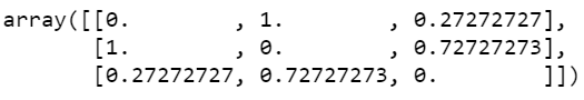

Normalized dissimilarity matrix

Second, we compute $S_{ij2}$ by DistanceMEtric.get_metric("manhattan"), and normalize it to the range 0 to 1: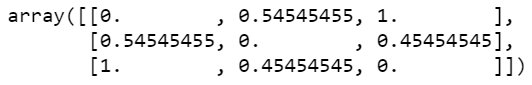

Normalized dissimilarity matrix

Third, we compute $S_{ij3}$. In this case, we have to compute the dice distance, since the third variable is a categorical variable. The dice distance is 0 whenever the values are equal, and 1 otherwise. The detailed computation of the dice distance can be found here. With DistanceMetric.get_metric("dice").pairwise(\alpha) where $\alpha$ refers to the data corresponding to 'Cat_1' that's converted into a numeric variable. Then, you get: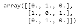

Dice distance of the categorical variable. Note that the categorical variable must've been converted into a numeric variable to run the dice distance

The final step is to add $S_{ij1}, S_{ij2}, S_{ij3}$ together, either using a simple mean or weighted mean. If we use the simple mean, the result is:

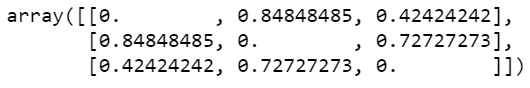
Dissimilarity matrix by the Gower's distance

The interpretation of the resulting dissimilarity matrix is:

• The distance between Row1 and Row2 is 0.84 and that of between Row1 and Row3 is 0.42.
• This means Row1 is more similar to Row3 compared to Row2. Intuitively, this makes sense as if we take a look at the dataset.

Application

You can apply hierarchical clustering (e.g. Agglomerative algorithm) to the resulting dissimilarity matrix. Refer to the steps of the agglomeration algorithm:

1. Create an initial set of clusters with each cluster consisting of a single record for all records in the data.
2. Compute the dissimilarity between all pairs of clusters.
3. Merge the two clusters that are least dissimilar as measured by the dissimilarity metric. $\rightarrow$ This is where we can utilize the dissimilarity matrix we computed by the Gower's distance.
4. Repeat steps 1-3 until we are left with one remaining cluster.

One Line Implementation

There is a python library, gower, to compute the Gower's distance. The implementation is one simple line: 

gower.gower_matrix(df)

 

Source: here