PyTorch Example of LSTM

Architecture [3]

The main components are: 1) hidden and cell states, 2) input gate, forget gate, output gate.

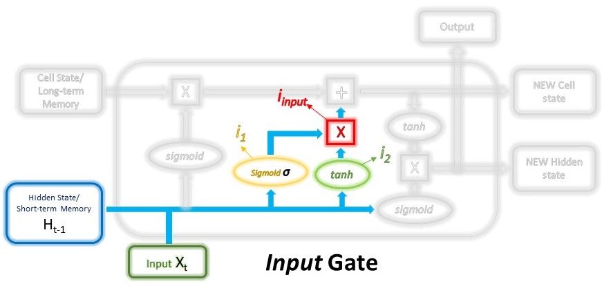
$$ i_1 = \sigma ( W_{i_1} \cdot (H_{t-1}, x_t) + b_{i_1} ) $$

$$ i_ = tanh ( W_{i_2} \cdot (H_{t-1}, x_t) + b_{i_2} ) $$

$$ i_{input} = i_1 * i_2 $$

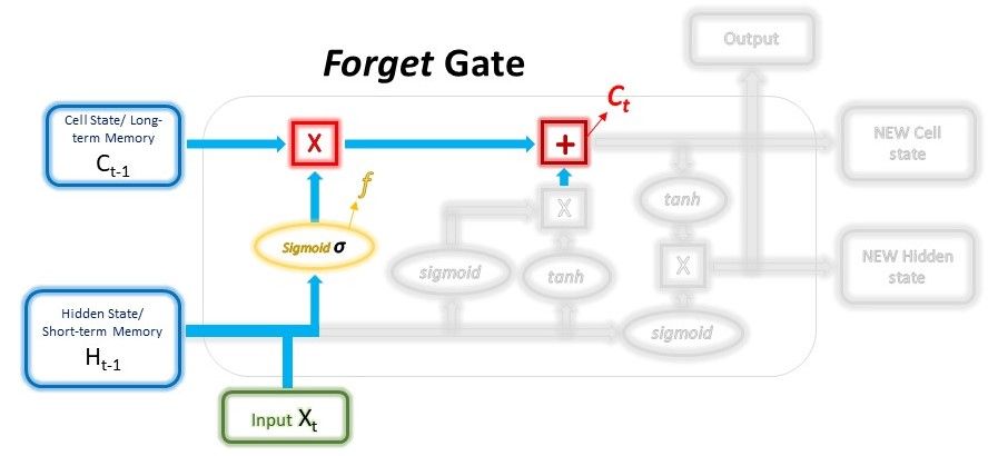
$$ f = \sigma ( W_{forget} \cdot (H_{t-1}, x_t) + b_{forget} ) $$

$$ C_t = C_{t-1} * f + i_{input} $$

$$ O_1 = \sigma ( W_{output_1} \cdot (H_{t-1}, x_t) + b_{output_1} ) $$

$$ O_2 = tanh ( W_{output_2} \cdot C_t + b_{output_2} ) $$

$$ H_t, O_t = O_1 * O_2 \tag{1} $$

In $Eq. (1)$, $H_t == Q_t$ is valid only when there is one LSTM layer.

PyTorch Example [1, 2, 4]

An LSTM model is trained to predict a gradient of first-order linear data. For example, if data is from $y=0.3 x$, the model should predict $0.3$.

Dataset

A (mini-)batch's dimension needs to be specially organized for LSTM as $(batch\_size, seq\_len, input\_size)$ if batch_first=True in nn.LSTM(..). Data from each linear function is organized as follows: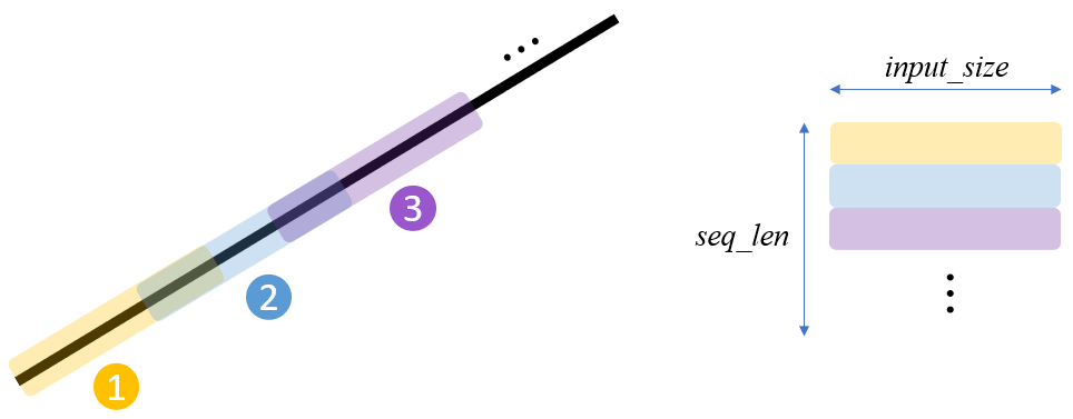

By fetching this stacked data over the batch dimension via DataLoder, we can obtain a training dataset for LSTM. Note that different linear gradients are used to stack along the batch dimension.

import numpy as np
import matplotlib.pyplot as plt

import torch
import torch.nn as nn
from torch.utils.data import Dataset, DataLoader


# generate a dataset

class MyDataset(Dataset):
    def __init__(self, n_grads, H):
        super().__init__()
        self.grads = np.random.uniform(-1, 1, size=n_grads)
        self.x = torch.arange(0, 1, 0.01)
        self.H = H # horizon [steps]
        self.interval = H//2 # [steps]

        self.len = n_grads

    def __getitem__(self, idx):
        """
        1. sample `grads`
        2. generate linear data (seq_len*input_size)
        Remarks: (batch_size*seq_len*input_size) is formed by DataLoader.
        """
        H = self.H

        # 1.
        grad = self.grads[idx]

        # 2.
        y = grad * self.x

        subys = torch.tensor([])  # (seq_len*input_size(H))
        i = 0
        while len(y[i:i+H]) == H:
            suby = y[i:i+H].view(1, -1)
            subys = torch.cat((subys, suby), 0)
            i += self.interval

        return subys, grad

    def __len__(self):
        return self.len

Model

The LSTM layer receives the mini-batch ($(batch\_size, seq\_len, input\_size)$) and yieds an output ($(batch\_size, seq\_len, hidden\_size)$). Then, we choose the last $output$ w.r.t the $seq\_len$ dimension, and it is fed into a linear layer for the regression task.

One important thing is to initialize the states (hidden and cell states) as zeros in the beginning w.r.t the $seq\_len$ dimension during training.

class LSTM(nn.Module):
    def __init__(self, in_size):
        super().__init__()
        self.in_size = in_size
        self.h_size = 32
        self.n_layers = 2

        # define the LSTM layer
        self.lstm = nn.LSTM(self.in_size, self.h_size, self.n_layers, 
                            batch_first=True)
        self.h_n = None  # hidden state
        self.c_n = None  # cell state

        # define the output layer
        self.linear = nn.Linear(self.h_size, 1)  # predicts `linear-grad`

    def init_states(self, batch_size):
        """initialize the hidden and cell states"""
        self.h_n = torch.zeros(self.n_layers, batch_size, self.h_size)
        self.c_n = torch.zeros(self.n_layers, batch_size, self.h_size)

    def forward(self, x):
        """
        x: (batch, seq_len, input_size)

        out: (batch, seq_len, hidden_size)
        h_n, c_n: (num_layers * num_directions, batch, hidden_size)
        """
        states = (self.h_n, self.c_n)
        out, (self.h_n, self.c_n) = self.lstm(x, states)

        # get the last one of the (sequential) output from the LSTM
        out = out[:, -1, :]  # (batch, hidden_size)
        out = self.linear(out)  # (batch, 1)

        return out

DataLoader & Model & Compile

# DataLoader
train_dataset = MyDataset(n_grads=30, H=10)
train_data_loader = DataLoader(train_dataset, batch_size=8)

val_dataset = MyDataset(n_grads=10, H=10)
val_data_loader = DataLoader(val_dataset, batch_size=8)


# Model
model = LSTM(in_size=train_dataset.H)


# Compile
optimizer = torch.optim.Adam(model.parameters(), lr=1e-3, weight_decay=1e-5)
criterion = nn.MSELoss()

Train

Note that .eval() or .train() are not used since there is no layer that requires that. Also, note that model.init_states(..) is used at the beginning of each mini-batch.

# Train
n_epochs = 100

for epoch in range(1, n_epochs+1):

    # train
    i, train_loss, val_loss = 0, 0., 0.
    for x, y in train_data_loader:
        optimizer.zero_grad()

        model.init_states(batch_size=x.shape[0])
        out = model(x)
        loss = criterion(out, y.float().view(-1, 1))
        train_loss += loss.item()

        loss.backward()
        optimizer.step()
        i += 1
    train_loss /= i

    # validate
    with torch.no_grad():
        i = 0
        for x, y in val_data_loader:
            model.init_states(batch_size=x.shape[0])
            out = model(x)
            loss = criterion(out, y.float().view(-1, 1))
            val_loss += loss.item()
            i += 1
        val_loss /= i

    print('epoch: {} | train_loss: {:0.5f} | val_loss: {:0.5f}'.format(epoch, train_loss, val_loss))

Results

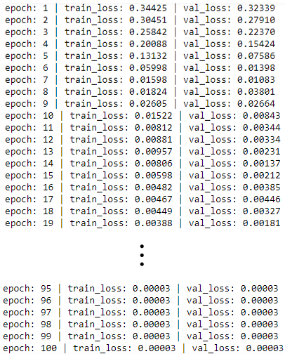
Training

Test

# Test
with torch.no_grad():
    for x, y in val_data_loader:
        model.init_states(batch_size=x.shape[0])
        out = model(x)
        break
        #loss = criterion(out, y.float().view(-1, 1))
        
# Plot
plt.plot(y.float(), 'o', label='y')
plt.plot(out.view(-1), '^', label='yhat')
plt.legend();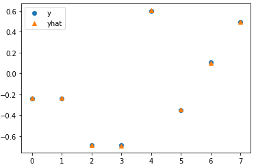

 

 

References

[1] Yung, J., 2018, "LSTMs for Time Series in PyTorch" (link)
[2] PyTorch LSTM example (link)
[3] Loye G., 2019, "Long Short-Term Memory: From Zero to Hero with PyTorch" (link)
[4] PyTorch: LSTM (link)