Variational Auto Encoder (VAE)

Reference: www.jeremyjordan.me/variational-autoencoders/

Variational autoencoders.

Key Concepts

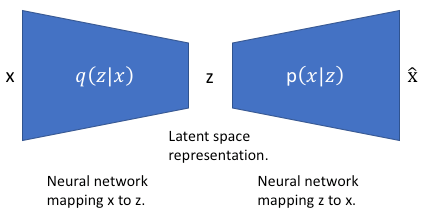
We define $x$, $z$ as input and latent representation, respectively, and a neural network for the VAE is modeled as follows:

Then, we'd like to compute the following conditional probability (distribution), $p(z | x)$ as posterior - the probability of observing $z$ when $x$ is given. This posterior can be separated by Bayes' theorem:

$$ p(z | x) = \frac{p(x|z) p(z)}{p(x)} $$

where $p(x|z)$ is likelihood, $p(z)$ is prior, and $p(x)$ is marginal. We do not really know how the real prior looks. It's likely that it is a complicated distribution than standard distributions such as a normal distribution. To approximate $p(z|x)$, we can utilize variation inference (VI). That is, 

$$ \mathrm{argmin}_{\lambda} KL[ q_{\lambda}(z|x) || p(z|x) ]  \tag{1}$$

where $\lambda \in \{ \mu_{\lambda_0}, \sigma_{\lambda_0}, \cdots \}$ is a variational parameter. By minimizing $Eq.(1)$, we can approximate the true posterior by the variational distribution. $Eq.(1)$ can be re-written as follows (link for full derivation; This derivation is also utilized in the book, "Probabilistic Deep Learning"): 

$$ \mathrm{argmax}_{\lambda} E_{q(z|x)} \log p(x|z) - KL[q_{\lambda}(z|x) || p(z) ]  \tag{2} $$

The first term represents the reconstruction likelihood and the second term ensures that our learned variational distribution $q$ is similar to the true prior distribution $p$. Commonly, a unit normal distribution is used for $p$. Finally, the loss function can be derived as follows:

$$ Loss = \mathcal{L}(x, \hat{x}) + \sum_j KL[ q_{\lambda_j}(z|x) || p(z) ] $$

where the first term penalizes reconstruction error (which can be thought of maximizing the reconstruction likelihood) and the second term which encourages our learned distribution $q(z|x)$ to be similar to the true prior distribution $p(z)$, which we'll assume follows a unit normal distribution, for each dimension j of the latent space.

$KL[q_{\lambda}(z|x) || p(z) ]$ can be written as 

$$ KL[q_{\lambda}(z|x) || p(z)] = - \frac{1}{2} \left[ 1 + \log(\sigma_q^2) - \sigma_q^2 - \mu_q^2 \right] $$

where $\mu_q$ and $\log(\sigma_q^2)$ ($\sigma^2$ is variance) are outputs from the encoder [1][2].

[1] S. Odaibo, "Variational Inference & Derivation of the Variational Autoencoder (VAE) Loss Function: A True Story", Medium (link)
[2] AntixK, "PyTorch-VAE", Github (link)

Implementation

In this example, we consider 2-dimensional latent embedding space composed of $z_0$ and $z_1$. Then, we need to define a multivariate normal distribution with a 2x2 covariance matrix:

\[ \Sigma = \begin{bmatrix} Cov(z_0, z_0) & Cov(z_0, z_1) \\ Cov(z_1, z_0) & Cov(z_1, z_1) \end{bmatrix} \]

However, we simplify the covariance matrix by assuming that the covariance matrix has zero values on non-diagonal terms. Therefore, only the diagonal terms have some values, which allows us to describe the covariance matrix with two values.

Note that exponential or softplus functions are applied to the variance terms to make them always positive.

In the figure, the latent embedding space is 2-dimensional and the variational parameters are:

$$ \boldsymbol{\lambda} = \{ \mu_{\lambda_0}, \sigma_{\lambda_0}, \mu_{\lambda_1}, \sigma_{\lambda_1} \} $$

$z_0$ and $z_1$ are originally sampled from normal distributions of $N( \mu_{\lambda_0}, \sigma_{\lambda_0} )$ and $N( \mu_{\lambda_1}, \sigma_{\lambda_1} )$, respectively. But, in that case, $z_0$ and $z_1$ are random variables, therefore, non-differentiable. To make them differentiable, we use the reparameterization trick:

$$ z = \mu + \sigma \epsilon; \;\; \epsilon \sim N(0,1) $$