[2021.03.09] Few-shot Learning; Self-supervised Learning

[Seminar Video] Metric-based Approaches to Meta-learning

Common Terminology regarding a Dataset for the Meta-learning

What is a Metric-based Approach to Meta-learning?

Metric-learning의 개념을 이용해서 meta-learning에 적용시킨 그런 방법론들을 지칭: Deep siamese network; Matching network; Protypical network; Relation network;

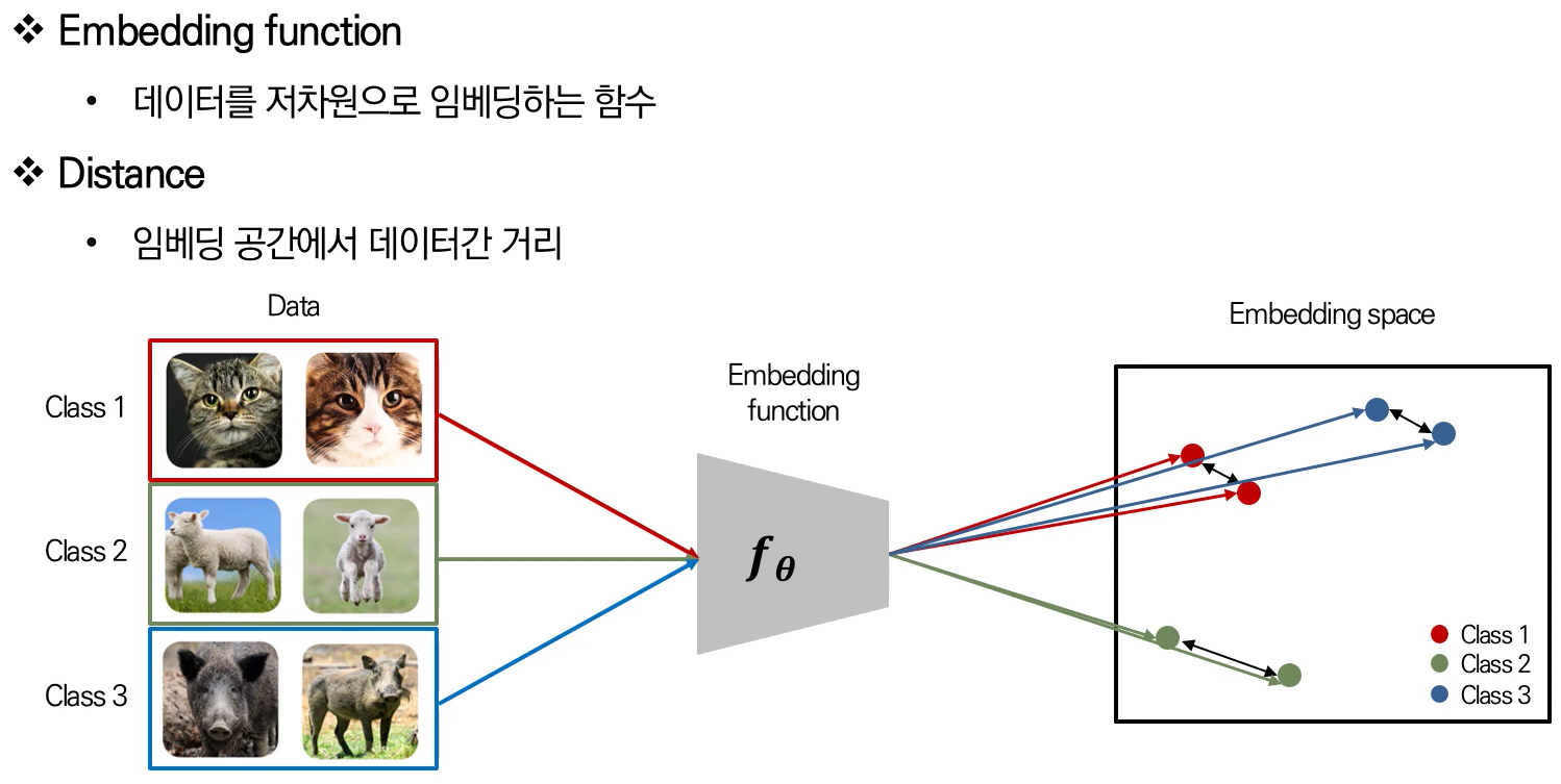
Metric-learning에 있어서 가장 중요한 개념 두가지: `Embedding function` and `Distance`. 위의 그림에서의 metric-learning은 embedding space상에서 같은 class끼리의 embedding vectors들은 가깝게, 다른 class끼리의 embedding vectors들은 서로 멀게 학습한다.

Reference: http://dmqm.korea.ac.kr/activity/seminar/301

G. Koch, et al., 2015, "Siamese Neural Networks for One-Shot Image Recognition"

- Metric-learning approach

The twin networks (entire weights are shared) take two different input (images) and output two representation vectors - $\boldsymbol{h}_1$ and $\boldsymbol{h}_2$. The two vectors are compared (merged) by a L1 distance metric, and the output probability $p$ is 1 if the two input images belong to the same class, if not, $p$ is zero. The training is conducted by minimizing the binary cross entropy of $p$. During the training, the representation vectors are learned. The detailed training procedure can be found in this PyTorch Siamese implementation on Github.

F. Sung, et al., 2017, "Matching Networks for One Shot Learning"

- Metric-learning approach

The previous version of the Prototypical network.

The model in its simplest form computes a predicted label $\hat{y}$ as follows:

$$ \hat{y} = \sum_{i=1}^{k} att( \hat{x}, x_i ) y_i \tag{1}$$

where $\hat{x}$, $x_i$, and $y_i$ are a test example, and samples and labels from the support set $S = \{ ( x_i, y_i ) \}_{i=1}^k$, respectively, and $att$ is an attention mechaism. Note that $Eq.(1)$ essentially describes the output for a new class as a linear combination of the labels in the support set. The attention value would be zero if $x_i$ and $\hat{x}$ are far away from each other and an appropirate constant otherwise. 

$Eq.(1)$ relies on choosing $att(. , .)$, which fully specifies the classifier. The simplest form is to use the softmax over the cosine distance $c$. That is,

$$ att(\hat{x}, x_i) = \frac{ \mathrm{exp}( c(f(\hat{x}), g(x_i)) ) }{ \sum_{j=1}^k \mathrm{exp}( c(f(\hat{x}), g(x_i)) ) } $$

where $f$ and $g$ are appropriate nueral networks (potentially $f=g$) to embed $\hat{x}$ and $x_i$.

The episodic training (episode-based training) was first proposed in this paper, which is well utilized for the Relation Network (F. Sung, 2018).

Episodic Training (Referred to from the Relation Network paper)

We consider the task of few-shot classifier learning. Formally, we have three datasets: a training set, a support set, and a testing set. The support set and testing set share the same label space, but the training set has its own label space that is disjoint with support/testing set. If the support set contains $K$ labelled examples for each of $C$ unique classes, the target few-shot problem is called $C$-way $K$-shot.

With the support set only, we can in principle train a classifier to assign a class label $\hat{y}$ to each sample $\hat{x}$ in the test set. However, due to the lack of labelled samples in the support set, the performance of such a classifier is usually not satisfactory. Therefore, we aim to perform meta-learning on the training set, in order to extract transferrable knowledge that will allow us to perform better few-shot learning on the support set and thus classify the test set more successfully.

An effective way to exploit the training set is to mimic the few-shot learning setting via episode-based training as proposed in this paper. In each training iteration, an episode is formed by randomly selecting $C$ classes from the training set with $K$ labelled samples from each of the $C$ classes to act as the sample set $\mathcal{S} = \{ (x_i, y_i) \}^m_{i=1}$ $(m=K \times C)$, as well as a fraction of the remainder of those $C$ classes' samples to serve as the query set $\mathcal{Q} = \{ (x_j, y_j) \}^n_{j=1}$ This sample/query set split is designed to simulate the support/test set that will be encountered at test time. 

J. Snell, et al., 2017, "Prototypical networks for few-shot learning"

- Metric-learning approach

This network is based on matching network, which uses an attention mechanism over a learned embedding of the labeled set of examples (the support set) to predict classes for the unlabeled points (the query set). The matching network can be interpreted as a weighted nearest-neighbor classifier applied within an embedding space.

The prototypical network is based on the idea that there exists an embedding in which points cluster around a single prototype representation for each class. In order to do this, we learn a non-linear mapping of the input into an embedding space using a neural network and take a class's prototype to be the mean of its support set in the embedding space. Classification is then performed for an embedded query point by simply finding the nearest class prototype. We follow the same approach to tackle zero-shot learning.

Learning Process

In few-shot classification, we are given a small support set of $N$ labeled examples $S=\{ (\boldsymbol{x}_1, y_1), \cdots, (\boldsymbol{x}_N, y_N) \}$ where each $\boldsymbol{x}_i \in \mathbb{R}^D$ is the $D$-dimensional feature vector of an example and $y_i \in \{ 1, \cdots, K \}$ is the corresponding label. $S_k$ denotes the set of examples labeled with class $k$.

Prototypical networks compute an $M$-dimensional representation $\boldsymbol{c}_k \in \mathbb{R}^M$, or prototype, of each class through an embedding function $f_{\phi} : \mathbb{R}^D \rightarrow \mathbb{R}^M$ with learnable parameters $\phi$. Each prototype is the mean vector of the embedded support points belonging to its class:

$$ \boldsymbol{c}_k = \frac{1}{ | S_k | }  \sum_{(\boldsymbol{x}_i, y_i) \in S_k}{f_{\phi}(\boldsymbol{x}_i) }$$

Given a distance function $d$, prototypical networks produce a distribution over classes for a query point $\boldsymbol{x}$ based on a softmax over distances to the prototypes in the embedding space:

$$ p_{\phi}(y=k | \boldsymbol{x}) = \frac{\mathrm{exp}(-d( f_{\phi}(\boldsymbol{x}), \boldsymbol{c}_k ))}{ \sum_k \mathrm{exp}( -d( f_{\phi}(\boldsymbol{x}), \boldsymbol{c}_k ) ) } $$

Learinng proceeds by minimizing the negative log-probability $J(\phi) = - log \; p_{\phi} (y = k | \boldsymbol{x})$ of the true class $k$ via SGD. Training episodes are formed by randomly selecting a subset of classes from the training set, then choosing a subset of examples within each class to act as the support set and a subset of the remainder to server as query points. Pseudocode to compute the loss $J(\phi)$ for a training episode is provided below:

It feels quite similar to the 'episodic training' as in Matching Network and Relation Network

S. Ravi, et al., 2017, "Optimization as a Model for Few-Shot Learning"

- Initialization-based Methods ∋ Learning an optimizer

In this paper, the authors proposed an LSTM-based meta-learner optimizer that is trained to optimize a learner neural network classifier. The meta-learner captures both short-term knowledge within a task and long-term knowledge common among all the tasks. By using an objective that directly captures an optimization algorithm's ability to have good generalization performance given only a set number of updates, the meta-learner model is trained to converge a learner classifier to a good solution quickly on each task. Additionally, the formulation of our meta-learner model allows it to learn a task-common initialization for the learner classifier, which captures fundamental knowledge shared among all the tasks.

In this paper, a configuration of the meta-learning dataset is similar to the prior papers:

The key idea of the LSTM-based meta learner is mimicking a process of gradient descent update with a parametric learning rate (with the input gate) and the forget gate for the learned weight introduced. The cell state in an LSTM is updated as:

$$ c_t = f_t \odot c_{t-1} + i_t \odot \tilde{c}_t \tag{1}$$

The $Eq.(1)$ is manipulated for the LSTM-based meta learner as in the following equation:

$$  c_t = f_t \odot \theta_{t-1} + i_t \odot ( - \nabla_{\theta_{t-1}} \mathcal{L}_t ) $$

where the $f_t$ and $i_t$ denote the forget gate and input gate, respectively, and $i_t$ acts as a parametric learning rate. $\theta_t$ denotes the parameters of the learner. The meta-learner get to determine optimal values of $i_t$ and $f_t$ through the course of the updates. The configurations of $i_t$ and $f_t$ are as follows:

$$ i_t = \sigma ( \boldsymbol{W}_I \cdot [ \nabla_{\theta_{t-1}} \mathcal{L}_t, \mathcal{L}_t, \theta_{t-1}, i_{t-1} ] + \boldsymbol{b}_I ) $$

$$ f_t = \sigma ( \boldsymbol{W}_F \cdot [ \nabla_{\theta_{t-1}} \mathcal{L}_t, \mathcal{L}_t, \theta_{t-1}, f_{t-1} ] + \boldsymbol{b}_F ) $$

With $i_t$, the meta-learner should be able to finely control the learning rate so as to train the learner quickly while avoiding divergence. As for $f_t$, what would justify shrinking the parameters of the learner and forgetting part of its previous value would be if the learner is currently in a bad local optima and needs a large change to escape. This would correspond to a situation where the loss is high but the gradient is close to zero. Additionally, notice that we can also learn the initial value of the cell state $c_0$ for the LSTM, treating it as a parameter of the meta-learner. This corresponds to the initial weights of the classifier. Learning this initial value lets the meta-learner determine the optimal initial weights of the learner so that training begins from a beneficial starting point that allows optimization to proceed rapidly.

F. Sung et al., 2018, "Learning to compare: Relation network for few-shot learning"

- Metric-learning approach

It is one of the metric-learning approaches to the meta-learning. The authors further aim to learn a transferrable deep metric for the few-shot learning or zero-shot learning instead of pred-defined fixed metric such as Euclidean. This Relation Net is most related to the prototypical network and siamese network, but it is an upgraded version.

The episodic training (episode-based training) is explicitly utilized, which was first proposed in the Matching Network paper.

The model of the Relation Network is illustrated in the following figure: 

One-shot

The relation network consists of two modules: an embedding module $f_{\varphi}$ and a relation module $g_{\phi}$. Samples $x_j$ in the query set $\mathcal{Q}$, and samples $x_i$ in the sample set $\mathcal{S}$ are fed through the embedding module $f_{\varphi}$, which produces feature maps $f_{\varphi}(x_i)$ and $f_{\varphi}(x_j)$. The feature maps $f_{\varphi}(x_i)$ and $f_{\varphi}(x_j)$ are combined with operator $\mathcal{C}$. In this work, we assume $C(\cdot, \cdot)$ to be concatenation of feature maps in depth, although other choices are possible.

The combined feature map of the sample and query are fed into the relation module $g_{\phi}$, which eventually produces a scalar in range of 0 to 1 representing the similarity between $x_i$ and $x_j$, which is called relation score, $r_{i, j}$. $r_{i, j}$ is for the relation between one query input $x_j$ and training sample set examples $x_i$.

$$ r_{i,j} = g_{\phi}( \mathcal{C} ( f_{\varphi}(x_i), f_{\varphi}(x_j) ) ); \;\;\; i=1,2, \cdots, C $$

K-shot

For K-shot where $K > 1$, we element-wise sum over the embedding module outputs of all samples from each training class to form this class' feature map. 

Objective Function

We use the MSE loss to train the model, regressing the relation score $r_{i, j}$ to the ground truth: matched pairs have similarity 1 and the mismatched pair have similarity 0.

$$ \varphi, \phi \leftarrow \mathrm{argmin}_{\varphi, \phi} \sum_{i=1}^m \sum_{j=1}^n ( r_{i,j} - \boldsymbol{1} (y_i == y_j) )^2 $$

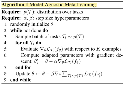
C. Finn et al., 2017, "Model-agnostic meta-learning for fast adaptation of deep networks" (MAML)

- Initialization-based Methods ∋ Good model initialization

It finds good initial weights by the meta-learner such that the weights can be adapted to the new task easily, fast, and efficiently:

A. Nicohl, 2018, "On first-order meta-learning algorithms" (Reptile)

- Initialization-based Methods ∋ Good model initialization

This paper proposes Reptile, a simplified version of the MAML, by considering only first-order derivatives for the meta-learning updates. The results show that the performance of the Reptile is very competitive to the MAML although it's the simplified version.

A. Rusu et al., 2019, "Meta-Learning with Latent Embedding Optimization"

- Initialization-based Methods ∋ Good model initialization

This paper proposes Latent Embedding Optimization (LEO). The LEO can be seen as an upgraded version of the MAML such that the LEO enables us to perform the MAML gradient-based adaptation steps in the learned, low-dimensional embedding space.

T. Munkhdalai et al., 2017, "Meta network"

The MetaNet consists of two main learning components: `a base learner` and `a meta learner` equipped with an external memory. The weights of the meta-learner are updated using the external memory.

The paper is not so comprehensible. Some notations are kinda confusing. I found no significant idea from this paper.

weight-update mechanism with the external memory